STAT 505 - Lesson 11 - Principal Component Analysis
Ramaa Nathan
4/3/2019
Data Exploration
Load File
places = read_table("data/places.txt", col_names=c("climate", "housing","health","crime","trans","educate","arts","recreate","econ","id") )
## Parsed with column specification:
## cols(
##   climate = col_integer(),
##   housing = col_integer(),
##   health = col_integer(),
##   crime = col_integer(),
##   trans = col_integer(),
##   educate = col_integer(),
##   arts = col_integer(),
##   recreate = col_integer(),
##   econ = col_integer(),
##   id = col_integer()
## )
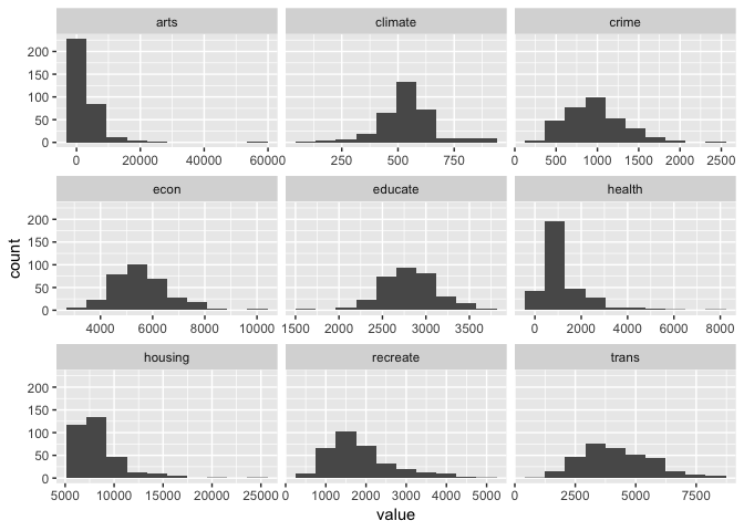
Plot histograms
ggplot(gather(places[,-10]),aes(value)) +
  geom_histogram(bins=10) +
  facet_wrap(~key, scales='free_x')
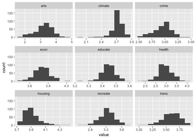
#apply log10 function - we do not need id here.. so remove it.
#places1 = places %>% select(-id) %>%
 # mutate_all(log10)
places1 <- places %>%
  mutate_at(vars(-id),log10)
ggplot(gather(places1[,-10]),aes(value)) +
  geom_histogram(bins=10) +
  facet_wrap(~key, scales='free_x')
formatAsTable <- function(df,title="Title") {
  #create the header vector
  table_header = ifelse(has_rownames(df),c(ncol(df)+1),c(ncol(df)))
  names(table_header)=c(title)
  #style the table
  df %>% kable() %>%
    kable_styling(full_width=F,bootstrap_options=c("bordered")) %>%
    add_header_above(table_header)
}
Principal Component Analysis using Covariance Matrix
Using princomp
#get the covariance matrix
places_cov <- cov(places1[,-10])
formatAsTable(data.frame(places_cov),"Covariance Matrix")
|
Covariance Matrix
|
|
|
climate
|
housing
|
health
|
crime
|
trans
|
educate
|
arts
|
recreate
|
econ
|
|
climate
|
0.0128923
|
0.0032678
|
0.0054793
|
0.0043741
|
0.0003857
|
0.0004415
|
0.0106886
|
0.0025733
|
-0.0009662
|
|
housing
|
0.0032678
|
0.0111161
|
0.0145962
|
0.0024831
|
0.0052786
|
0.0010696
|
0.0292263
|
0.0091270
|
0.0026458
|
|
health
|
0.0054793
|
0.0145962
|
0.1027279
|
0.0099550
|
0.0211535
|
0.0074778
|
0.1184844
|
0.0152994
|
0.0014634
|
|
crime
|
0.0043741
|
0.0024831
|
0.0099550
|
0.0286107
|
0.0072989
|
0.0004713
|
0.0319466
|
0.0092847
|
0.0039464
|
|
trans
|
0.0003857
|
0.0052786
|
0.0211535
|
0.0072989
|
0.0248289
|
0.0024619
|
0.0470407
|
0.0115675
|
0.0008344
|
|
educate
|
0.0004415
|
0.0010696
|
0.0074778
|
0.0004713
|
0.0024619
|
0.0025200
|
0.0095204
|
0.0008772
|
0.0005465
|
|
arts
|
0.0106886
|
0.0292263
|
0.1184844
|
0.0319466
|
0.0470407
|
0.0095204
|
0.2971732
|
0.0508600
|
0.0062060
|
|
recreate
|
0.0025733
|
0.0091270
|
0.0152994
|
0.0092847
|
0.0115675
|
0.0008772
|
0.0508600
|
0.0353078
|
0.0027924
|
|
econ
|
-0.0009662
|
0.0026458
|
0.0014634
|
0.0039464
|
0.0008344
|
0.0005465
|
0.0062060
|
0.0027924
|
0.0071365
|
#compute PCA
pr_cov <- princomp(places1[,-10],cor=FALSE,scores=TRUE,fix_sign=TRUE)
summary(pr_cov)
## Importance of components:
##                           Comp.1     Comp.2    Comp.3     Comp.4
## Standard deviation     0.6134452 0.22560372 0.1668374 0.15131845
## Proportion of Variance 0.7226740 0.09774248 0.0534537 0.04397184
## Cumulative Proportion  0.7226740 0.82041652 0.8738702 0.91784205
##                            Comp.5     Comp.6     Comp.7      Comp.8
## Standard deviation     0.12930691 0.10916208 0.09182048 0.062627954
## Proportion of Variance 0.03210956 0.02288413 0.01619086 0.007532295
## Cumulative Proportion  0.94995161 0.97283574 0.98902660 0.996558897
##                             Comp.9
## Standard deviation     0.042330504
## Proportion of Variance 0.003441103
## Cumulative Proportion  1.000000000
#eigen values = variance = (pr_cov$sdev)^2
# create a dataframe with eigen values, differences, variance of proportion and ciumulative proportion of variance
proportionOfVar = data_frame(EigenValue=(pr_cov$sdev)^2,
                             Difference=EigenValue-lead(EigenValue),
                             Proportion=EigenValue/sum(EigenValue),
                             Cumulative=cumsum(EigenValue)/sum(EigenValue))
formatAsTable(proportionOfVar,"Variances / Eigen Values")
|
Variances / Eigen Values
|
|
EigenValue
|
Difference
|
Proportion
|
Cumulative
|
|
0.3763151
|
0.3254180
|
0.7226740
|
0.7226740
|
|
0.0508970
|
0.0230623
|
0.0977425
|
0.8204165
|
|
0.0278347
|
0.0049374
|
0.0534537
|
0.8738702
|
|
0.0228973
|
0.0061770
|
0.0439718
|
0.9178421
|
|
0.0167203
|
0.0048039
|
0.0321096
|
0.9499516
|
|
0.0119164
|
0.0034854
|
0.0228841
|
0.9728357
|
|
0.0084310
|
0.0045087
|
0.0161909
|
0.9890266
|
|
0.0039223
|
0.0021304
|
0.0075323
|
0.9965589
|
|
0.0017919
|
NA
|
0.0034411
|
1.0000000
|
#get the loadings - the Eigen Vectors
eigenVectors = pr_cov$loadings;
#create a dataframe - only for display purposes
eigenVectorsDF <- data.frame(matrix(eigenVectors,9,9))
row.names(eigenVectorsDF) <- unlist(dimnames(eigenVectors)[1])
colnames(eigenVectorsDF) <- unlist(dimnames(eigenVectors)[2])
formatAsTable(eigenVectorsDF,"Eigen Vectors")
|
Eigen Vectors
|
|
|
Comp.1
|
Comp.2
|
Comp.3
|
Comp.4
|
Comp.5
|
Comp.6
|
Comp.7
|
Comp.8
|
Comp.9
|
|
climate
|
0.0350729
|
0.0088782
|
0.1408748
|
0.1527448
|
0.3975116
|
0.8312950
|
0.0559096
|
0.3149012
|
0.0644892
|
|
housing
|
0.0933516
|
0.0092306
|
0.1288497
|
-0.1783823
|
0.1753133
|
0.2090573
|
-0.6958923
|
-0.6136158
|
-0.0868770
|
|
health
|
0.4077645
|
-0.8585319
|
0.2760577
|
-0.0351614
|
0.0503247
|
-0.0896708
|
0.0624528
|
0.0210358
|
0.0655033
|
|
crime
|
0.1004454
|
0.2204237
|
0.5926882
|
0.7236630
|
-0.0134571
|
-0.1640189
|
0.0555304
|
-0.1823479
|
-0.0542122
|
|
trans
|
0.1500971
|
0.0592011
|
0.2208982
|
-0.1262053
|
-0.8699695
|
0.3724496
|
-0.0724604
|
0.0571420
|
0.0718394
|
|
educate
|
0.0321532
|
-0.0605886
|
0.0081447
|
-0.0051969
|
-0.0477977
|
0.0236280
|
-0.0573857
|
0.2044731
|
-0.9732711
|
|
arts
|
0.8743406
|
0.3038063
|
-0.3632873
|
0.0811157
|
0.0550699
|
-0.0281215
|
0.0232698
|
0.0167399
|
0.0052566
|
|
recreate
|
0.1589962
|
0.3339926
|
0.5836260
|
-0.6282261
|
0.2132899
|
-0.1417991
|
0.2345152
|
0.0835391
|
-0.0174947
|
|
econ
|
0.0194942
|
0.0561011
|
0.1208534
|
0.0521700
|
0.0296524
|
-0.2648128
|
-0.6644859
|
0.6620318
|
0.1682638
|
#Display the scores of the first 10 observations
pr_cov$scores %>% head(10) %>% formatAsTable(.,"Scores")
|
Scores
|
|
Comp.1
|
Comp.2
|
Comp.3
|
Comp.4
|
Comp.5
|
Comp.6
|
Comp.7
|
Comp.8
|
Comp.9
|
|
-0.4366771
|
0.4201634
|
-0.1181209
|
0.0899588
|
-0.0809683
|
0.0050283
|
-0.0777766
|
0.1428702
|
0.0029877
|
|
0.6209576
|
0.0053458
|
0.0018082
|
-0.1007449
|
0.0216497
|
0.0272882
|
0.1347766
|
-0.0276786
|
0.0677809
|
|
-0.8732563
|
-0.2121036
|
0.0496929
|
0.1716117
|
0.0266537
|
-0.0444182
|
-0.0442839
|
-0.0659487
|
0.0096433
|
|
0.5029481
|
-0.0636215
|
-0.1704949
|
-0.1123026
|
-0.1963132
|
0.0455147
|
-0.0308016
|
0.0872710
|
-0.0364262
|
|
0.6097750
|
-0.0072326
|
0.2331267
|
0.0502339
|
-0.0711925
|
0.0596135
|
0.0472725
|
0.0467325
|
-0.0009515
|
|
-0.7456332
|
-0.1881828
|
-0.0407524
|
0.0727651
|
0.0636872
|
-0.0271343
|
0.0403322
|
0.0547203
|
-0.0354845
|
|
0.0050971
|
0.0634965
|
-0.3781554
|
-0.0250161
|
0.0958425
|
0.0581775
|
-0.0427086
|
0.0153939
|
-0.0566308
|
|
-0.0393760
|
-0.0923854
|
-0.0952791
|
0.0044039
|
-0.1235088
|
0.0517066
|
0.0066959
|
0.1004058
|
0.0085536
|
|
-0.8935752
|
-0.0978617
|
-0.1070677
|
-0.2011014
|
-0.1240106
|
0.1701246
|
0.0600887
|
0.0422251
|
-0.0047487
|
|
-0.1649041
|
0.0417715
|
-0.0279384
|
0.1843475
|
-0.1220699
|
0.0822534
|
-0.0294404
|
0.0902523
|
0.0106447
|
pr_cov_combined <- cbind(places1,pr_cov$scores)
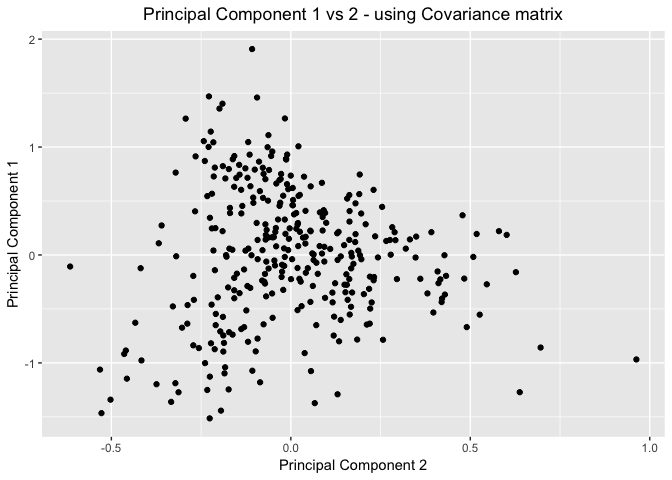
Scatter Plots of the Principal Components - using Covariance Matrix
#Plot the first two principal components
data.frame(pr_cov_combined) %>%
  ggplot(mapping=aes(x=Comp.2,y=Comp.1)) +
  geom_point() +
  #geom_text(aes(label=id,hjust=0,vjust=0)) +
  labs(title = "Principal Component 1 vs 2 - using Covariance matrix") +
  theme(plot.title = element_text(hjust = 0.5))+
  xlab("Principal Component 2") +
  ylab("Principal Component 1")
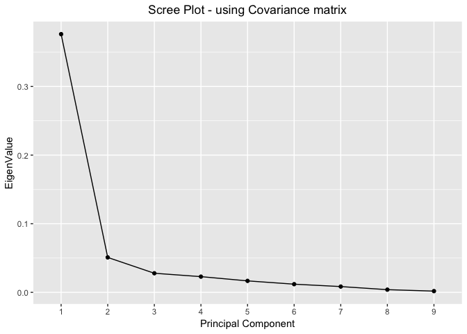
Scree Plots - using Covariance Matrix
proportionOfVar %>%
  ggplot(mapping=aes(x=seq(nrow(proportionOfVar)),y=EigenValue))+
  geom_point()+
  geom_line()+
  scale_x_discrete(limits=seq(nrow(proportionOfVar))) +
  xlab("Principal Component") +
  labs(title="Scree Plot - using Covariance matrix") +
  theme(plot.title = element_text(hjust = 0.5))
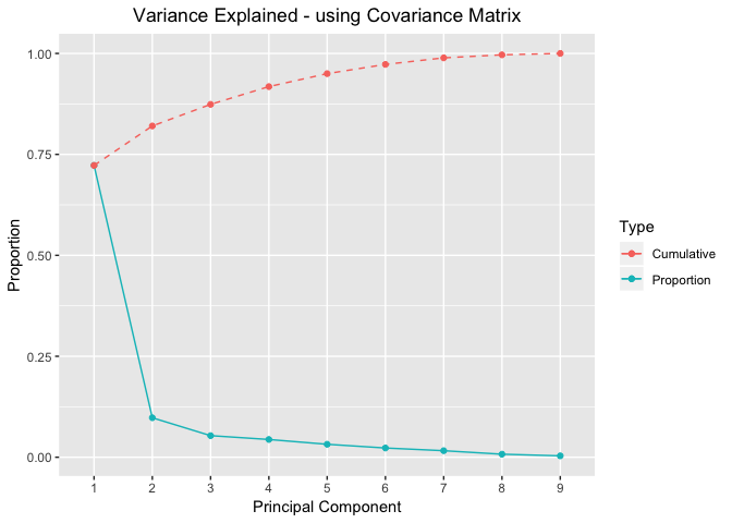
Variance Explained Plots - using Covariance Matrix
 proportionOfVar %>%
  ggplot(mapping=aes(x=seq(nrow(proportionOfVar)))) +
  geom_point(aes(y=Proportion,colour="red"))+
  geom_line(aes(y=Proportion,colour="red"))+
  geom_point(aes(y=Cumulative,colour="blue"))+
  geom_line(aes(y=Cumulative,colour="blue"),linetype="dashed")+
  scale_color_discrete(name="Type",labels=c("Cumulative","Proportion"))+ #legend
  scale_x_discrete(limits=seq(nrow(proportionOfVar))) + #xlabel
  xlab("Principal Component") +
  labs(title="Variance Explained - using Covariance Matrix") +
  theme(plot.title = element_text(hjust = 0.5))
Correlation between Principal Components and Variables -using Covariance Matrix
# select only the first three principal components (so ignore column id and all columns named Comp.4 to Comp.9)
 pr_cov_combined %>% select(-matches("*.[4-9]$"),-id) %>%
  cor() %>% as.data.frame() %>%
  select(starts_with("Comp")) %>%
  formatAsTable(.,"Correlation between Principal Components and Variables")
|
Correlation between Principal Components and Variables
|
|
|
Comp.1
|
Comp.2
|
Comp.3
|
|
climate
|
0.1897764
|
0.0176671
|
0.2073107
|
|
housing
|
0.5439783
|
0.0197815
|
0.2042024
|
|
health
|
0.7816315
|
-0.6052287
|
0.1439164
|
|
crime
|
0.3648400
|
0.2944431
|
0.5854860
|
|
trans
|
0.5852356
|
0.0848904
|
0.2342438
|
|
educate
|
0.3935162
|
-0.2727092
|
0.0271101
|
|
arts
|
0.9854003
|
0.1259213
|
-0.1113525
|
|
recreate
|
0.5198621
|
0.4016138
|
0.5189836
|
|
econ
|
0.1417745
|
0.1500496
|
0.2390394
|
|
Comp.1
|
1.0000000
|
0.0000000
|
0.0000000
|
|
Comp.2
|
0.0000000
|
1.0000000
|
0.0000000
|
|
Comp.3
|
0.0000000
|
0.0000000
|
1.0000000
|
Using prcomp
#compute PCA using prcomp - (SVD method)
#IMPORTANT - when using prcomp, always set center=TRUE to match the results from princomp with covaraince matrix
pr_cov2 <- prcomp(places1[,-10],scale=FALSE,center=TRUE)

#eigen values = variance = (pr_cov$sdev)^2
# create a dataframe with eigen values, differences, variance of proportion and ciumulative proportion of variance
proportionOfVar = data_frame(EigenValue=(pr_cov2$sdev)^2,
                             Difference=EigenValue-lead(EigenValue),
                             Proportion=EigenValue/sum(EigenValue),
                             Cumulative=cumsum(EigenValue)/sum(EigenValue))
formatAsTable(proportionOfVar,"Variances / Eigen Values")
|
Variances / Eigen Values
|
|
EigenValue
|
Difference
|
Proportion
|
Cumulative
|
|
0.3774624
|
0.3264102
|
0.7226740
|
0.7226740
|
|
0.0510522
|
0.0231326
|
0.0977425
|
0.8204165
|
|
0.0279196
|
0.0049525
|
0.0534537
|
0.8738702
|
|
0.0229671
|
0.0061958
|
0.0439718
|
0.9178421
|
|
0.0167713
|
0.0048186
|
0.0321096
|
0.9499516
|
|
0.0119527
|
0.0034960
|
0.0228841
|
0.9728357
|
|
0.0084567
|
0.0045225
|
0.0161909
|
0.9890266
|
|
0.0039342
|
0.0021369
|
0.0075323
|
0.9965589
|
|
0.0017973
|
NA
|
0.0034411
|
1.0000000
|
#get the laodings - the Eigen Vectors
eigenVectors = pr_cov2$rotation;
#create a dataframe - only for display purposes
eigenVectorsDF <- data.frame(matrix(eigenVectors,9,9))
row.names(eigenVectorsDF) <- unlist(dimnames(eigenVectors)[1])
colnames(eigenVectorsDF) <- unlist(dimnames(eigenVectors)[2])
formatAsTable(eigenVectorsDF,"Eigen Vectors")
|
Eigen Vectors
|
|
|
PC1
|
PC2
|
PC3
|
PC4
|
PC5
|
PC6
|
PC7
|
PC8
|
PC9
|
|
climate
|
0.0350729
|
0.0088782
|
-0.1408748
|
0.1527448
|
-0.3975116
|
0.8312950
|
-0.0559096
|
-0.3149012
|
-0.0644892
|
|
housing
|
0.0933516
|
0.0092306
|
-0.1288497
|
-0.1783823
|
-0.1753133
|
0.2090573
|
0.6958923
|
0.6136158
|
0.0868770
|
|
health
|
0.4077645
|
-0.8585319
|
-0.2760577
|
-0.0351614
|
-0.0503247
|
-0.0896708
|
-0.0624528
|
-0.0210358
|
-0.0655033
|
|
crime
|
0.1004454
|
0.2204237
|
-0.5926882
|
0.7236630
|
0.0134571
|
-0.1640189
|
-0.0555304
|
0.1823479
|
0.0542122
|
|
trans
|
0.1500971
|
0.0592011
|
-0.2208982
|
-0.1262053
|
0.8699695
|
0.3724496
|
0.0724604
|
-0.0571420
|
-0.0718394
|
|
educate
|
0.0321532
|
-0.0605886
|
-0.0081447
|
-0.0051969
|
0.0477977
|
0.0236280
|
0.0573857
|
-0.2044731
|
0.9732711
|
|
arts
|
0.8743406
|
0.3038063
|
0.3632873
|
0.0811157
|
-0.0550699
|
-0.0281215
|
-0.0232698
|
-0.0167399
|
-0.0052566
|
|
recreate
|
0.1589962
|
0.3339926
|
-0.5836260
|
-0.6282261
|
-0.2132899
|
-0.1417991
|
-0.2345152
|
-0.0835391
|
0.0174947
|
|
econ
|
0.0194942
|
0.0561011
|
-0.1208534
|
0.0521700
|
-0.0296524
|
-0.2648128
|
0.6644859
|
-0.6620318
|
-0.1682638
|
#Display the scores of the first 10 observations
pr_cov2$x %>% head(10) %>% formatAsTable(.,"Scores")
|
Scores
|
|
PC1
|
PC2
|
PC3
|
PC4
|
PC5
|
PC6
|
PC7
|
PC8
|
PC9
|
|
-0.4366771
|
0.4201634
|
0.1181209
|
0.0899588
|
0.0809683
|
0.0050283
|
0.0777766
|
-0.1428702
|
-0.0029877
|
|
0.6209576
|
0.0053458
|
-0.0018082
|
-0.1007449
|
-0.0216497
|
0.0272882
|
-0.1347766
|
0.0276786
|
-0.0677809
|
|
-0.8732563
|
-0.2121036
|
-0.0496929
|
0.1716117
|
-0.0266537
|
-0.0444182
|
0.0442839
|
0.0659487
|
-0.0096433
|
|
0.5029481
|
-0.0636215
|
0.1704949
|
-0.1123026
|
0.1963132
|
0.0455147
|
0.0308016
|
-0.0872710
|
0.0364262
|
|
0.6097750
|
-0.0072326
|
-0.2331267
|
0.0502339
|
0.0711925
|
0.0596135
|
-0.0472725
|
-0.0467325
|
0.0009515
|
|
-0.7456332
|
-0.1881828
|
0.0407524
|
0.0727651
|
-0.0636872
|
-0.0271343
|
-0.0403322
|
-0.0547203
|
0.0354845
|
|
0.0050971
|
0.0634965
|
0.3781554
|
-0.0250161
|
-0.0958425
|
0.0581775
|
0.0427086
|
-0.0153939
|
0.0566308
|
|
-0.0393760
|
-0.0923854
|
0.0952791
|
0.0044039
|
0.1235088
|
0.0517066
|
-0.0066959
|
-0.1004058
|
-0.0085536
|
|
-0.8935752
|
-0.0978617
|
0.1070677
|
-0.2011014
|
0.1240106
|
0.1701246
|
-0.0600887
|
-0.0422251
|
0.0047487
|
|
-0.1649041
|
0.0417715
|
0.0279384
|
0.1843475
|
0.1220699
|
0.0822534
|
0.0294404
|
-0.0902523
|
-0.0106447
|
Principal Component Analysis using Correlation Matrix - Standardized values
—————————————————————————
#compute PCA
pr_corr <- princomp(places1[,-10],cor=TRUE,scores=TRUE,fix_sign=TRUE)
summary(pr_corr)
## Importance of components:
##                           Comp.1    Comp.2    Comp.3    Comp.4     Comp.5
## Standard deviation     1.8159827 1.1016178 1.0514418 0.9525124 0.92770076
## Proportion of Variance 0.3664214 0.1348402 0.1228367 0.1008089 0.09562541
## Cumulative Proportion  0.3664214 0.5012617 0.6240983 0.7249072 0.82053259
##                            Comp.6     Comp.7     Comp.8     Comp.9
## Standard deviation     0.74979050 0.69557215 0.56397886 0.50112689
## Proportion of Variance 0.06246509 0.05375785 0.03534135 0.02790313
## Cumulative Proportion  0.88299767 0.93675552 0.97209687 1.00000000
#eigen values = variance = (pr_corr$sdev)^2
# create a dataframe with eigen values, differences, variance of proportion and ciumulative proportion of variance
proportionOfVar = data_frame(EigenValue=(pr_corr$sdev)^2,
                             Difference=EigenValue-lead(EigenValue),
                             Proportion=EigenValue/sum(EigenValue),
                             Cumulative=cumsum(EigenValue)/sum(EigenValue))
formatAsTable(proportionOfVar,"Variances / Eigen Values")
|
Variances / Eigen Values
|
|
EigenValue
|
Difference
|
Proportion
|
Cumulative
|
|
3.2977930
|
2.0842311
|
0.3664214
|
0.3664214
|
|
1.2135619
|
0.1080320
|
0.1348402
|
0.5012617
|
|
1.1055299
|
0.1982500
|
0.1228367
|
0.6240983
|
|
0.9072798
|
0.0466512
|
0.1008089
|
0.7249072
|
|
0.8606287
|
0.2984429
|
0.0956254
|
0.8205326
|
|
0.5621858
|
0.0783652
|
0.0624651
|
0.8829977
|
|
0.4838206
|
0.1657485
|
0.0537578
|
0.9367555
|
|
0.3180722
|
0.0669440
|
0.0353414
|
0.9720969
|
|
0.2511282
|
NA
|
0.0279031
|
1.0000000
|
#get the laodings - the Eigen Vectors
eigenVectors = pr_corr$loadings;
#create a dataframe - only for display purposes
eigenVectorsDF <- data.frame(matrix(eigenVectors,9,9))
row.names(eigenVectorsDF) <- unlist(dimnames(eigenVectors)[1])
colnames(eigenVectorsDF) <- unlist(dimnames(eigenVectors)[2])
formatAsTable(eigenVectorsDF,"Eigen Vectors")
|
Eigen Vectors
|
|
|
Comp.1
|
Comp.2
|
Comp.3
|
Comp.4
|
Comp.5
|
Comp.6
|
Comp.7
|
Comp.8
|
Comp.9
|
|
climate
|
0.1579414
|
0.0686294
|
0.7997100
|
0.3768095
|
0.0410459
|
0.2166950
|
0.1513516
|
0.3411282
|
0.0300976
|
|
housing
|
0.3844053
|
0.1392088
|
0.0796165
|
0.1965430
|
-0.5798679
|
-0.0822201
|
0.2751971
|
-0.6061010
|
-0.0422691
|
|
health
|
0.4099096
|
-0.3718120
|
-0.0194754
|
0.1125221
|
0.0295694
|
-0.5348756
|
-0.1349750
|
0.1500575
|
0.5941276
|
|
crime
|
0.2591017
|
0.4741325
|
0.1284672
|
-0.0422996
|
0.6921710
|
-0.1399009
|
-0.1095036
|
-0.4201255
|
0.0510119
|
|
trans
|
0.3748890
|
-0.1414864
|
-0.1410683
|
-0.4300767
|
0.1914161
|
0.3238914
|
0.6785670
|
0.1188325
|
0.1358433
|
|
educate
|
0.2743254
|
-0.4523553
|
-0.2410558
|
0.4569430
|
0.2247437
|
0.5265827
|
-0.2620958
|
-0.2111749
|
-0.1101242
|
|
arts
|
0.4738471
|
-0.1044102
|
0.0110263
|
-0.1468813
|
0.0119302
|
-0.3210571
|
-0.1204986
|
0.2598673
|
-0.7467268
|
|
recreate
|
0.3534118
|
0.2919424
|
0.0418164
|
-0.4040189
|
-0.3056537
|
0.3941388
|
-0.5530938
|
0.1377181
|
0.2263654
|
|
econ
|
0.1640135
|
0.5404531
|
-0.5073103
|
0.4757801
|
-0.0371078
|
-0.0009737
|
0.1468669
|
0.4147736
|
0.0479028
|
#Display the scores of the first 10 observations
pr_corr$scores %>% head(10) %>% formatAsTable(.,"Scores")
|
Scores
|
|
Comp.1
|
Comp.2
|
Comp.3
|
Comp.4
|
Comp.5
|
Comp.6
|
Comp.7
|
Comp.8
|
Comp.9
|
|
-1.2006820
|
1.4766156
|
-0.9457658
|
0.5570233
|
0.6763275
|
0.9534051
|
0.5379046
|
0.9569135
|
-0.7331827
|
|
0.9397421
|
-0.2488284
|
1.1075997
|
-1.6593654
|
-0.4120841
|
-0.7082161
|
-0.1965465
|
0.4896324
|
0.1473423
|
|
-2.3510699
|
0.3402471
|
0.0254193
|
0.6504602
|
0.3985502
|
-0.7400013
|
0.2592204
|
-0.7342527
|
0.4057979
|
|
1.3813627
|
-1.6161980
|
-1.2566714
|
0.1791818
|
0.0709811
|
0.8077640
|
0.5482947
|
0.6379999
|
-0.2998302
|
|
2.4410789
|
0.1918855
|
0.4155578
|
-0.2652699
|
0.9842905
|
0.4233625
|
0.0518763
|
0.2991611
|
0.4111207
|
|
-2.2402408
|
-0.6174960
|
-0.1048217
|
1.0862646
|
0.6134955
|
0.2211733
|
-0.5226177
|
0.1447510
|
0.1780500
|
|
-0.7942163
|
-1.2712570
|
0.0429201
|
1.1490846
|
-0.6843994
|
0.2985075
|
-0.1242866
|
0.0421718
|
-1.0540174
|
|
-0.2909512
|
-0.7283306
|
-0.4695213
|
0.2576317
|
0.5141451
|
0.3432275
|
0.5418614
|
0.8721576
|
0.0197242
|
|
-2.4455798
|
-1.5105915
|
0.4667603
|
-0.3331633
|
-0.5294227
|
1.1769692
|
0.6609870
|
0.4987692
|
0.2474489
|
|
-0.3418286
|
0.2615801
|
-0.0695413
|
0.5731232
|
1.2578601
|
0.3166650
|
0.8770192
|
0.6150955
|
-0.1289547
|
pr_corr_combined <- cbind(places1,pr_corr$scores)
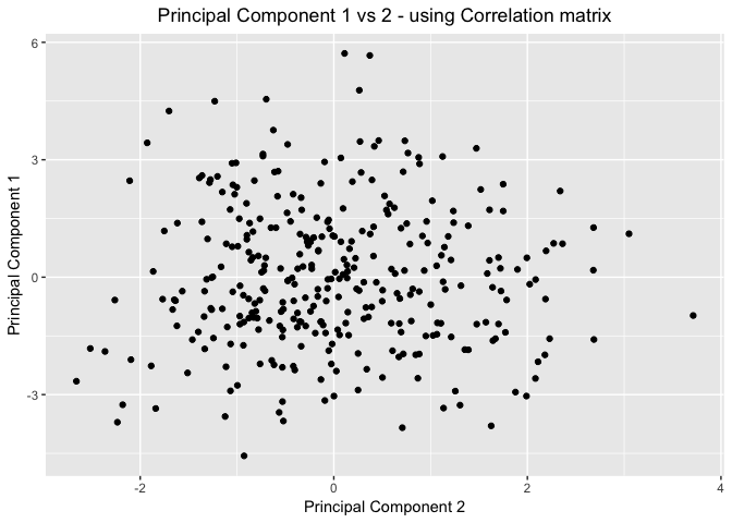
Scatter Plots of the Principal Components - using Correlation Matrix
#Plot the first two principal components
data.frame(pr_corr_combined) %>%
  ggplot(mapping=aes(x=Comp.2,y=Comp.1)) +
  geom_point() +
  #geom_text(aes(label=id,hjust=0,vjust=0)) +
  labs(title = "Principal Component 1 vs 2 - using Correlation matrix") +
  theme(plot.title = element_text(hjust = 0.5))+
  xlab("Principal Component 2") +
  ylab("Principal Component 1")
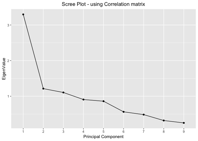
Scree Plots - using Correlation Matrix
proportionOfVar %>%
  ggplot(mapping=aes(x=seq(nrow(proportionOfVar)),y=EigenValue))+
  geom_point()+
  geom_line()+
  scale_x_discrete(limits=seq(nrow(proportionOfVar))) +
  xlab("Principal Component") +
  labs(title="Scree Plot - using Correlation matrix") +
  theme(plot.title = element_text(hjust = 0.5))
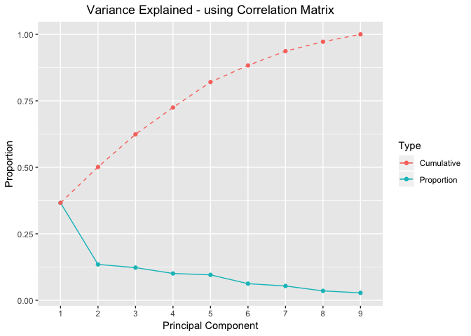
Variance Explained Plots -using Correlation Matrix
 proportionOfVar %>%
  ggplot(mapping=aes(x=seq(nrow(proportionOfVar)))) +
  geom_point(aes(y=Proportion,colour="red"))+
  geom_line(aes(y=Proportion,colour="red"))+
  geom_point(aes(y=Cumulative,colour="blue"))+
  geom_line(aes(y=Cumulative,colour="blue"),linetype="dashed")+
  scale_color_discrete(name="Type",labels=c("Cumulative","Proportion"))+ #legend
  scale_x_discrete(limits=seq(nrow(proportionOfVar))) + #xlabel
  xlab("Principal Component") +
  labs(title="Variance Explained - using Correlation Matrix") +
  theme(plot.title = element_text(hjust = 0.5))
Correlation between Principal Components and Variables - using Correlation Matrix
# select only the first three principal components (so ignore column id and all columns named Comp.4 to Comp.9)
 pr_corr_combined %>% select(-matches("*.[4-9]$"),-id) %>%
  cor() %>% as.data.frame() %>%
  select(starts_with("Comp")) %>%
  formatAsTable(.,"Correlation between Principal Components and Variables")
|
Correlation between Principal Components and Variables
|
|
|
Comp.1
|
Comp.2
|
Comp.3
|
|
climate
|
0.2868188
|
0.0756033
|
0.8408485
|
|
housing
|
0.6980733
|
0.1533549
|
0.0837121
|
|
health
|
0.7443888
|
-0.4095948
|
-0.0204772
|
|
crime
|
0.4705242
|
0.5223128
|
0.1350758
|
|
trans
|
0.6807920
|
-0.1558640
|
-0.1483251
|
|
educate
|
0.4981701
|
-0.4983226
|
-0.2534562
|
|
arts
|
0.8604980
|
-0.1150201
|
0.0115935
|
|
recreate
|
0.6417896
|
0.3216090
|
0.0439675
|
|
econ
|
0.2978456
|
0.5953728
|
-0.5334072
|
|
Comp.1
|
1.0000000
|
0.0000000
|
0.0000000
|
|
Comp.2
|
0.0000000
|
1.0000000
|
0.0000000
|
|
Comp.3
|
0.0000000
|
0.0000000
|
1.0000000
|